A Microscope into the Dark Matter of Interpretability
We propose a new interpretability architecture that learns a hierarchy of features in LLMs.
Too Long; Didn't Read
We propose the RQAE (Residual Quantization Autoencoder), a new architecture to interpret LLM representations which learns features hierarchically. You can control the specificity of a feature as you move through the hierarchy, and can naturally split features into more specific subfeatures. In evaluations, RQAE has better reconstruction than SAEs, and we find that RQAE features are more interpretable than Gemmascope SAE features using Eleuther AI's evaluation suite.
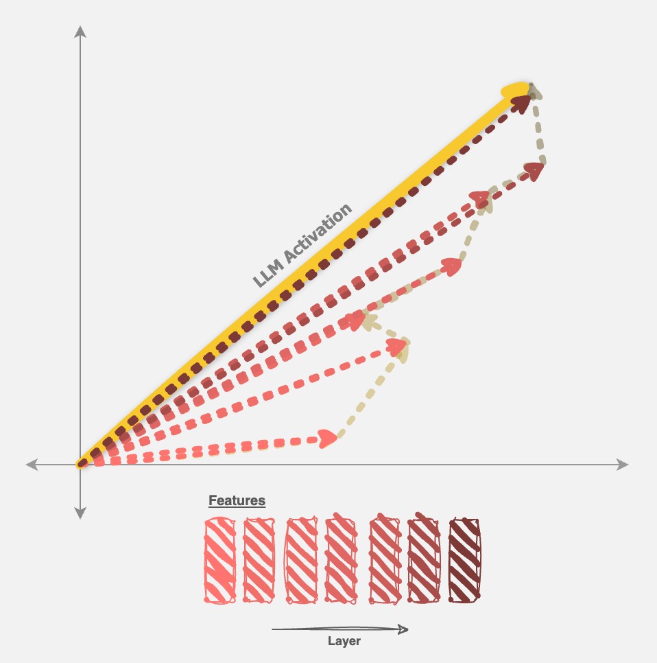
A single layer of RQAE projects the activation of a LLM into a learned (very small) subspace, quantizes the subspace, and projects back to the original dimension. Then, the residual between the original activation and this quantized representation is the input to the next layer. Each layer learns a new subspace, which depends on the previous residual, so later layers are dependent on earlier layers. This induces a hierarchy.
A recent paper finds that the residuals of SAEs (i.e. original activation - SAE reconstruction) contain extra features that even the largest SAEs do not find. RQAE reduces these pathological errors iteratively. Since we can show that vector quantization is a specific type of SAE, RQAE can be equivalently defined as stacking many (weak) SAEs on top of each other.
This post presents the motivation, architecture, and experiments justifying RQAE. We also have released the code, model weights, and a feature dashboard.
Introduction
The purpose of interpretability is to decompose a model into human-understandable features. This focus has led to some incredibly interesting work, such as include visualizing what parts of an image a model uses to predict a class
However, Large Language Models (LLMs) may be more complicated to interpret. Text is a much denser interpretable medium than visuals, and LLMs are orders of magnitude larger than any other model we’ve ever trained. This work is heavily inspired by transformer-circuits, which has laid out a foundation for how we can begin to interpret LLMs. If you’re new to interpretability, we would recommend reading these works first, but we’ll provide a quick rundown of the core concepts in the sections below.
Other work has explored how different layers of the LLM contribute to different functions (for example, the feedforward layers store facts and “knowledge”
World Models
What is a human interpretable feature, and why would they exist in LLMs? We know that LLMs store “world models” because they are really good at predicting the next token, and compressing the training data to the extent that they do requires some latent understanding of the world. Other work explores this concept in detail
- There are a large number of things that can happen in the world
- We observe what happens, and we reason about what happens with a much smaller set of “latent” features.
For example, if we see someone drop a glass bottle, then we expect the bottle to shatter when it hits the ground. This is not because we have observed exactly that person dropping exactly that bottle before. It’s because we have learned a very small set of latent features about physics, which we can use to model the bottle breaking.
LLMs must do something similar - they just don’t have the capacity to fully memorize their training data! Thus, they must also be working with some set of latent features that they can manipulate to solve the next token prediction task. A lot of interpretability research is focused on finding these latent features, and figuring out how the model uses them.
Linear Representations and Superposition
How do LLMs organize and use these latent features? There’s a lot of empirical evidence that LLMs describe features as simply directions in space, known as the Linear Representation Hypothesis (LRH). If true, it’s a very powerful framework - directions are just vectors, and we have a lot of theory to work with vectors.
Then, a full LLM activation is the sum of multiple atomic feature vectors. For example, we might think of a dog as the ‘animal’ feature plus the ‘pet’ feature, minus the ‘feline’ feature. Features also scale differently depending on the subject: a dog will have more of the ‘smart’ feature than a goldfish.
We borrow a formal definition of the LRH from here:
Definition 1: A linear representation has the following two properties:The Linear Representation Hypothesis states that an LLM linearly represents human-interpretable features.
- Composition as Addition: The presence of a feature is represented by adding that feature.
- Intensity as Scaling: The intensity of a feature is represented by magnitude.
There is one problem with the LRH: the residual stream of an LLM with width $d$ lies in the space $\mathbb{R}^d$. However, there can be at most $d$ orthogonal vectors in this space (the basis of the space), which means that there can be at most $d$ unique “feature directions”.
In order for the LRH to be true, models must learn features in superposition. This means that features interfere with each other, and you can not fully separate all features (e.g. any token with feature X must also have at least a little bit of feature Y, even if they’re two distinct features). However, you can also fit exponentially more features in a $d$-dimensional space which are only $\epsilon$-orthogonal to each other!
Similar features take similar directions, so interference is usually okay. Thus, when measuring by cosine similarity, we see clusters forming which correspond to similar features. For example, the “has fur” feature should be more aligned with the “cat” feature than with the “shark” feature - although in this example, interference might make it hard for the model to learn what a hairless cat is.
Sparse Autoencoders
Sparse Autoencoders (SAEs) model the LRH by learning an overcomplete basis to take features out of superposition
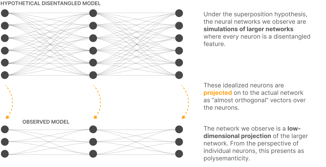
Thinking back to World Models, this actually makes a lot of sense! We can think of the “larger” model as the set of disentangled latent features that model the real world. The larger model only activates sparsely - only some neurons are activated for any given input. Sparse autoencoders try to reconstruct this larger model, in order to represent features out of superposition.
Definition 2: A sparse autoencoder $S$ of size $n$ is a model that takes in a LLM activation $r \in \mathbb{R}^d$ and does the following: $$ C(r) = \sigma(W_{in}r + b_{in}) $$ $$ S(r) = W_{out}C(r) +b_{out} $$ where $\sigma$ is some nonlinearity (usually ReLU), and $W_{out} \in \mathbb{R}^{d \times n}, W_{in} \in \mathbb{R}^{n \times d}$ (for $n \gg d$). $b_{in} \in \mathbb{R}^n, b_{out} \in \mathbb{R}^d$ are bias terms. The model is trained to minimize the reconstruction error $||r - S(r)||_2$. An additional loss term is added to induce sparsity in $C(r)$ - common methods to induce sparsity include TopK, L1 loss , or learning a threshold per feature .
To explicitly draw the connection to the LRH, a SAE performs the following algorithm (ignoring biases):
- Begin with some entangled LLM activation $r$, and consider that $W_{in}$ consists of $n$ “encoding” vectors.
- Compare $r$ against each encoding vector by calculating their dot product.
- Apply a nonlinearity (usually ReLU) and some sparsity function (TopK, L1, etc.), to act as a filter for sparsity.
- There are now $n$ coefficients $C(r) = [c_1, c_2, …]$, which are the intensities of each feature in $r$.
- Multiply $C$ by the columns of $W_{out}$, which are the actual feature vectors (“decoding” vectors) that you have learned.
However, an SAE can only learn a set number $n$ of features, and it’s likely that $n \ll N$ for the true number of features $N$ the LLM has learned. To give an example, consider two “ground-truth” features $f_1$ and $f_2$ - these features are similar but not exactly the same (e.g. different breeds of dogs). How will the SAE learn these features?
The Feature Hierarchy
The rough answer to the question posed above is: the model will learn an average direction that will fire weakly for these features - for example, a “dog” feature. It might also learn a few features that weakly activate for related, more general features - for example, a “living” feature, or a “pet” feature. Empirically, SAEs only learn general features, and more specific features are indistinguishable from one another.
There are two widely observed issues with SAEs that stem from this intuition:
- Feature splitting. If you train a wider SAE, you will notice that more general features split into smaller, more specific features.
-
Feature absorption. You learn two separate features in your SAE that are describing the same ground-truth feature - as a result, representations with that ground-truth feature are split across the two learned features without any discernable pattern (the difference between the two features is completely spurious)
.
The reason these happen is because SAE features are not necessarily atomic. They might need to be broken down or grouped together, but it’s difficult to tell which is which, and the training objective doesn’t bias the model one way or the other. This begs the question: how should we organize features?
A paper from UChicago attempts to answer this question
SAEs treats features as if they are all categorical. It can learn hierarchies of features (for example, it can learn separate features for organism, plant, animal, etc.) - but there is nothing in the architecture that encourages it to learn such features. Our best guess is that it learns hierarchy based on the frequency of the concepts in the training data alone, based on other work
Adding Inductive Bias
As mentioned above, SAEs do not have an inductive bias for how features should relate to one another. At the end of training, you are left with a flat dictionary of features, and it is up to you to interpret and organize them.
In contrast, this work introduces the inductive bias that features must be composed hierarchically. It’s not clear whether hierarchy is sufficient or necessary for all features a LLM represents, but feature hierarchies do seem like the natural answer to solving the problem of feature splitting/absorption.
We define a feature hierarchy to consist of parent and child features, such that any time a feature is activated, it’s parent will also be activated, and zero or one of it’s children will be activated. This addresses the two issues presented in the previous section:
- If a feature splits, then we define the base feature as higher in the hierarchy, and the split features as lower in the hierarchy.
- If two features should be absorbed, then only consider their common parent feature as the atomic feature.
This isn’t the only way to define a feature hierarchy (and probably not the best way) - for example, you can define a many-to-many relationship between parents and children - but it is simple and, as shown in the next section, easy to implement.
RQAE
In this section, we present the Residual Quantization Autoencoder (RQAE).
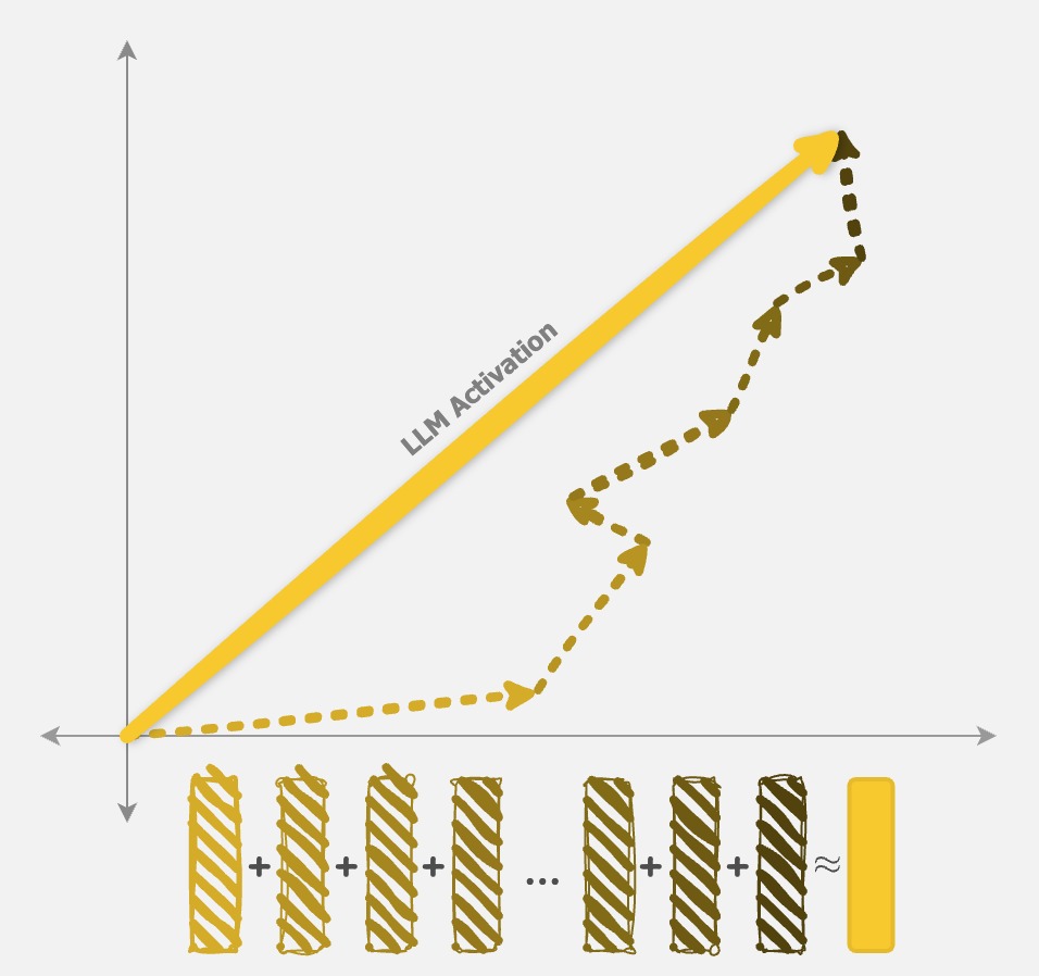
Since RQAE tackles the same problem as SAEs (decomposing an activation into interpretable parts), it should be no surprise that the end result also looks similar. Fig 1a shows how both RQAE and SAE split up an activation from an LLM. We even use the same training loss (MSE)!
Of course, not all feature decompositions are equal. SAE relies on the bottleneck of sparsity to control the type of features that are learned. RQAE uses two bottlenecks: projecting into subspaces, and quantizing the subspaces into a relatively small number of codebooks (i.e. only a few directions in the subspace can be chosen).
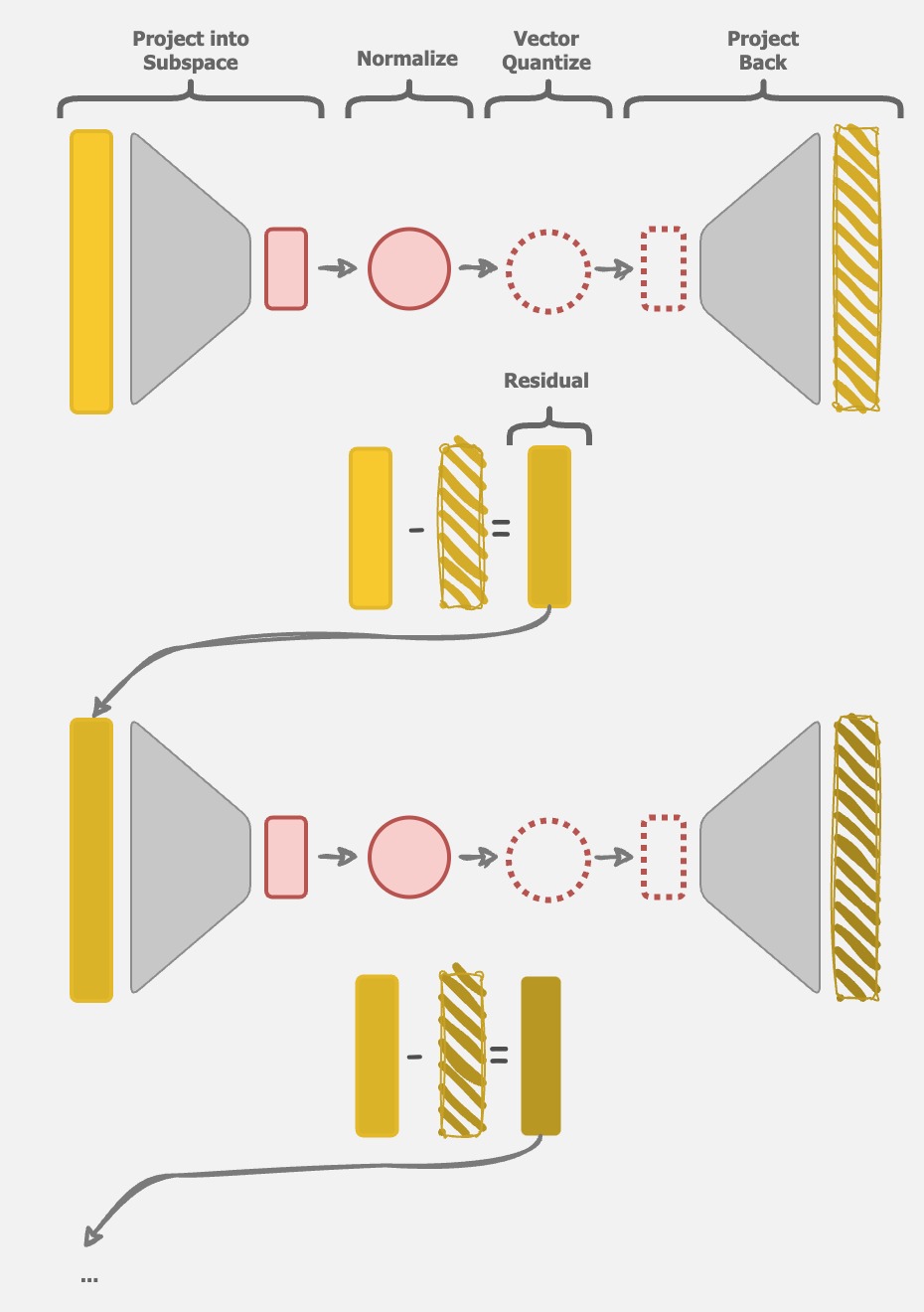
RQAE uses residual vector quantization
<span id="algo">
Here is the equivalent algorithm (to SAEs) for RQAE:
- Begin with some LLM activation $r$. For $n_q$ layers, repeat the following:
- Project $r$ into a small subspace with a linear layer, called projection $p$.
- Normalize $p$ to get $p_{norm}$
- Find the closest codebook to $p_{norm}$ from a set of codebooks using Euclidean distance. Call this codebook $\hat p$, with index $c_i$ for layer $i$.
- Project $\hat p$ back into the activation space with a linear layer, called $\hat r$.
- Set $r = r - \hat r$ as the residual.
- The original activation $r$ has now been quantized with $n_q$ codebooks, and can be represented as a set of codebook indices $(c_1, c_2, …, c_{n_q})$
Similar to how a SAE models the LRH, RQAE models the “feature hierarchy” mentioned above. For any given LLM activation, every layer chooses exactly one codebook. The subspaces that later layers choose are dependent on earlier layers (since the input to any given layer is original activation - sum(quantizations from previous layers)), encouraging a learned hierarchy between layers. Thus, a RQAE model with $n$ layers and $c$ codebooks per layer learns $c \times n$ unique values, but can represent $c^n$ different activations.
RQAE = Stacked SAEs
We draw a connection between the layers of a RQAE and a SAE.
Conceptually, a single layer of RQAE consists of the same parts as the SAE algorithm mentioned above: an encoder (linear in layer), intensity coefficients (codebook values), and a decoder that corresponds to features (linear out layer). Formally:
Lemma 1: A single layer of RQAE can be equivalently defined as a Top1 SAE.
Proof: Still a WIP. Will follow this work closely
In practice, we use a very small codebook dimension (in the experiments section, $4$). This is needed for vector quantization (especially FSQ, whose codebook size grows exponentially with respect to codebook dimension). At first glance, this seems concerning: a SAE can find features in a feature manifold that lives in higher-dimensional subspaces, but a RQAE layer can not!
This is true theoretically. However, in practice there is a large body of work that suggests LLM features and feature manifolds are mostly represented in very low dimensional subspaces (i.e. they are rank deficient)
Why quantization?
A natural question to ask is why quantization should be used in the first place. Especially if quantization = weak SAE, why not just use a better SAE? We don’t think quantization is necessary, and would be interested in future work that replicates RQAE using SAEs instead of quantization!
However, quantization turns out to be very useful:
- Quantization (= Top1 SAE) allows only a 1:1 parent:child relationship. It’s not clear how to define a hierarchy with a TopK SAE where $K > 1$ efficiently. One option could be to only consider the highest $N$ activating sets of features for any input activation.
- RVQ is a very well-studied field. As a result, there are many techniques already developed to help quantization. For example, it seemed to take the community several months to handle “dead features” in SAEs. RVQ has a handful of techniques that are empirically investigated across multiple domains to solve the problem of uniform codebook usage. Also, this problem becomes exponentially harder with more layers, so we’re not sure how SAEs will properly address it.
- Quantization models are more than an order of magnitude smaller than SAEs. RQAE, which provides much better reconstruction than even the largest Gemmascope SAE with the highest L0, is also smaller than the smallest available Gemmascope SAE.
Modeling Dark Matter
Previous work shows that SAEs learn pathological errors
Interestingly, even the largest SAEs that were evaluated (1 million features) still miss a significant portion of total (linear) features found in the LLM (Figure 10a
How would one fix this issue with SAEs alone? If you assume that sparse coding is enough of an inductive bias to find interpretable features at very high SAE sizes
This work provides a great motivation for RQAE! A single layer of RQAE is equivalent to a (weak) SAE, as shown above. The next layer of RQAE then learns on the residuals of the first layer, which we assume to have “missing features”, since reconstruction is not perfect. Applying this iteratively allows us to learn more “missing” features after each layer. This mimics the exact experiment run in the paper
In the next section we show that RQAE empirically also reduces reconstruction error (i.e. higher capacity) compared to even very large SAEs, as expected.
Training a Model
We train a RQAE with $n_q=1024$ layers, and use a codebook dimension of $d=4$ with quantized values of $[-1, -0.5, 0, 0.5, 1]$ per dimension - resulting in $544$ codebooks per layer (see FSQ
| Parameter | Value | Description |
|---|---|---|
| LLM | Gemma 2 2B | Base model to interpret |
| Layer | Residual Stream after the center layer (12) | What layer of the residual stream to train on |
| Training Data | FineWeb-Edu | Dataset used to train RQAE |
| Test Data | pile-uncopyrighted (Neuronpedia subset) | Dataset used for analysis |
| num_tokens | 1B | How many tokens we train on |
| context_length | 128 | Context length we train on |
We normalize activations passed into RQAE by using the final RMS norm layer of the LLM (note that this means all activations have exactly the same norm). Ablations are still a WIP, but will be added soon.
Let’s look at properties of learned model, to validate assumptions we have based on the model architecture.
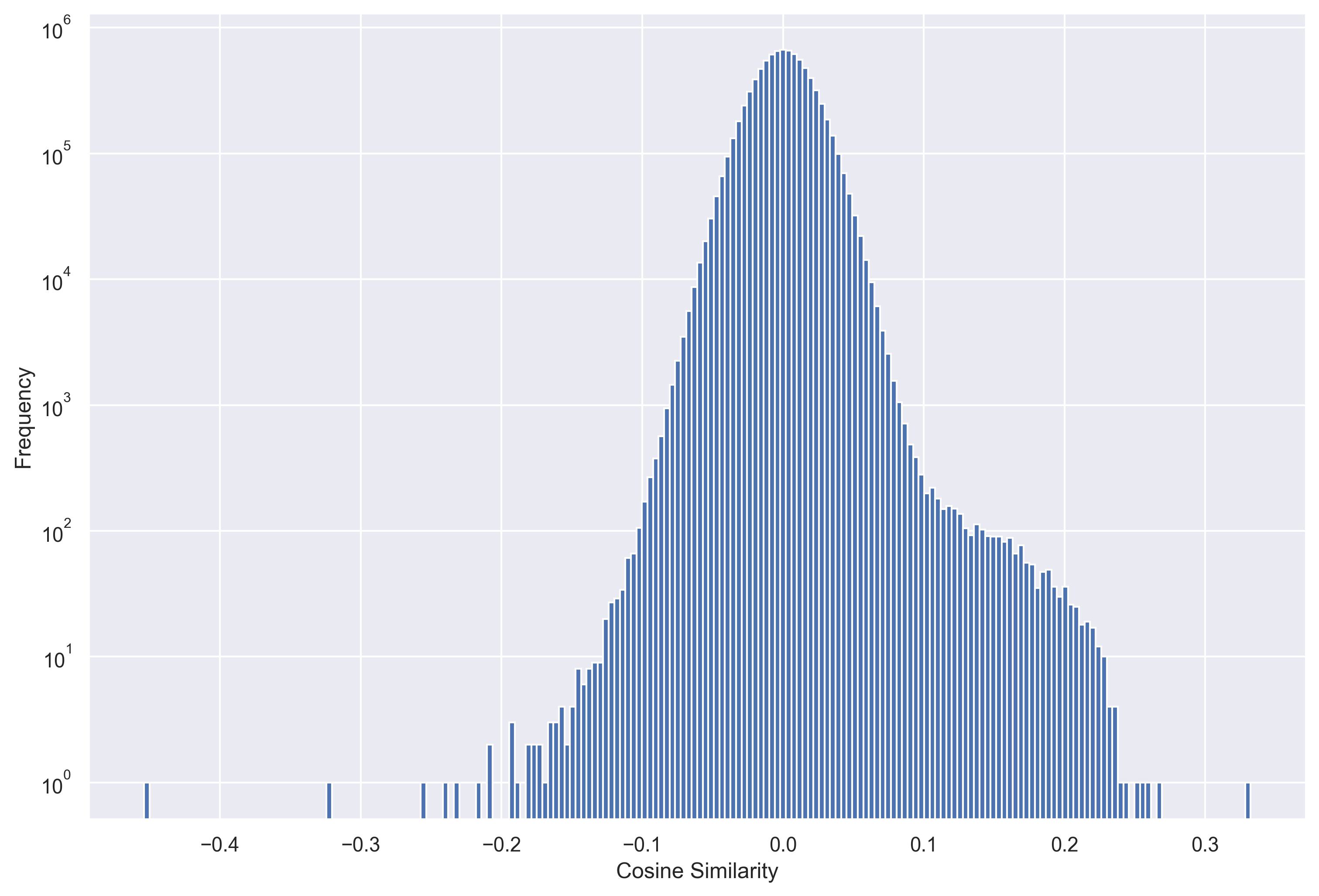
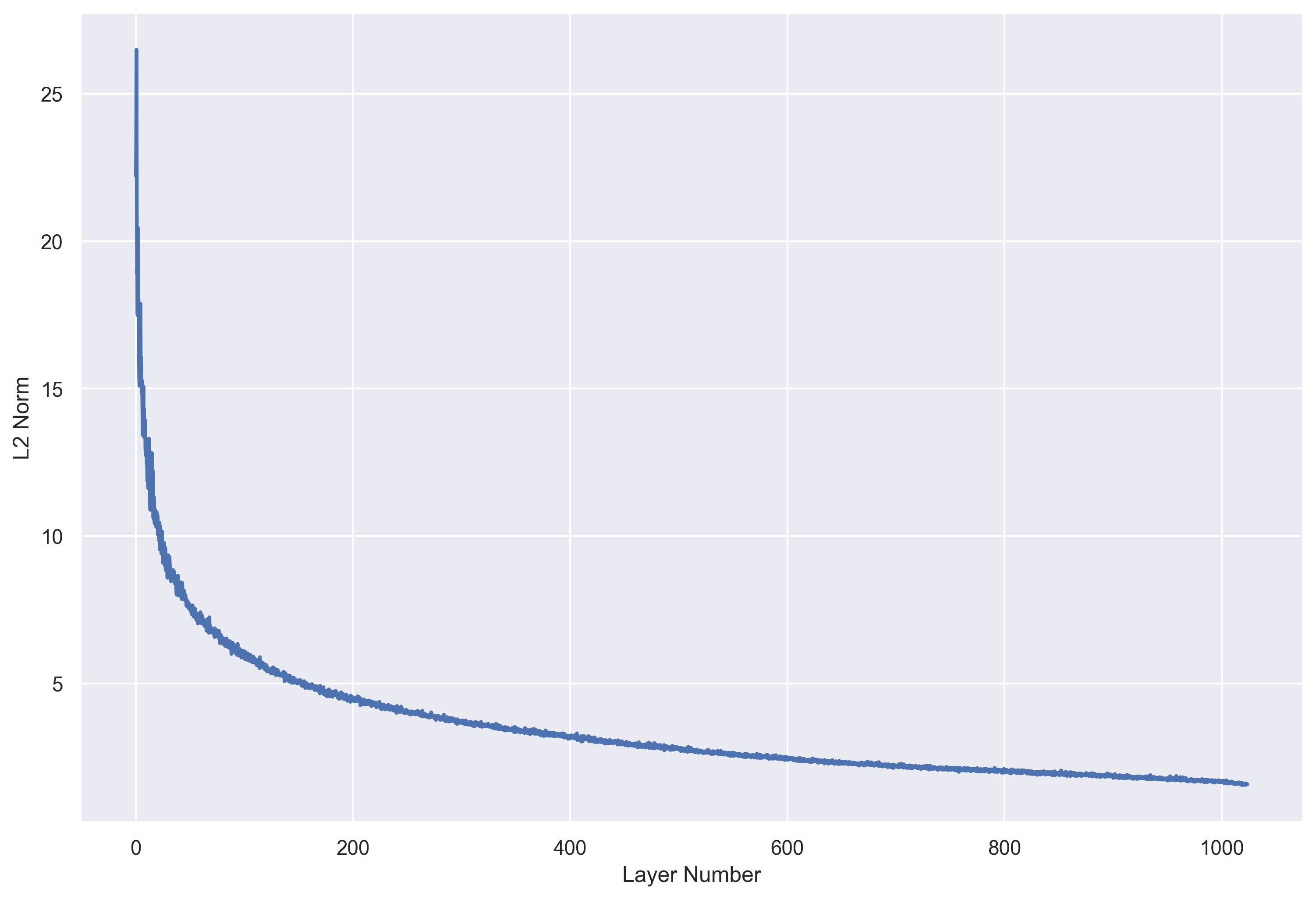
Figure 2a shows the distribution of pairwise cosine similarities between all projected codebooks. Almost all projected codebooks are $\epsilon$-orthogonal with $\epsilon=0.2$, suggesting that they form an overcomplete basis. It also shows the L2 norm of features across RQAE layers - earlier layers have larger norms than later layers, suggesting that earlier layers choose more “confident” directions, and the majority of MSE loss is concentrated in the first few layers.
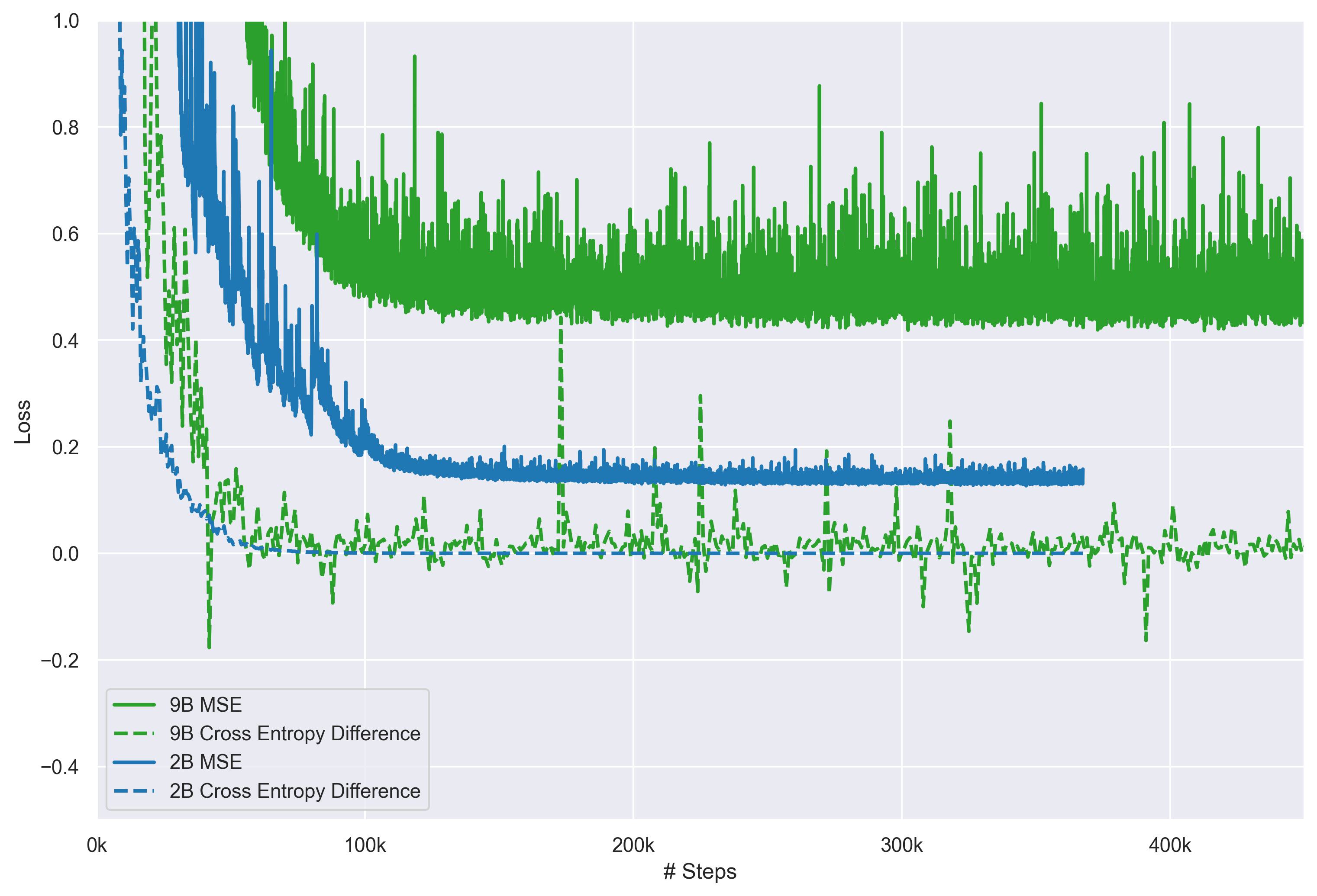
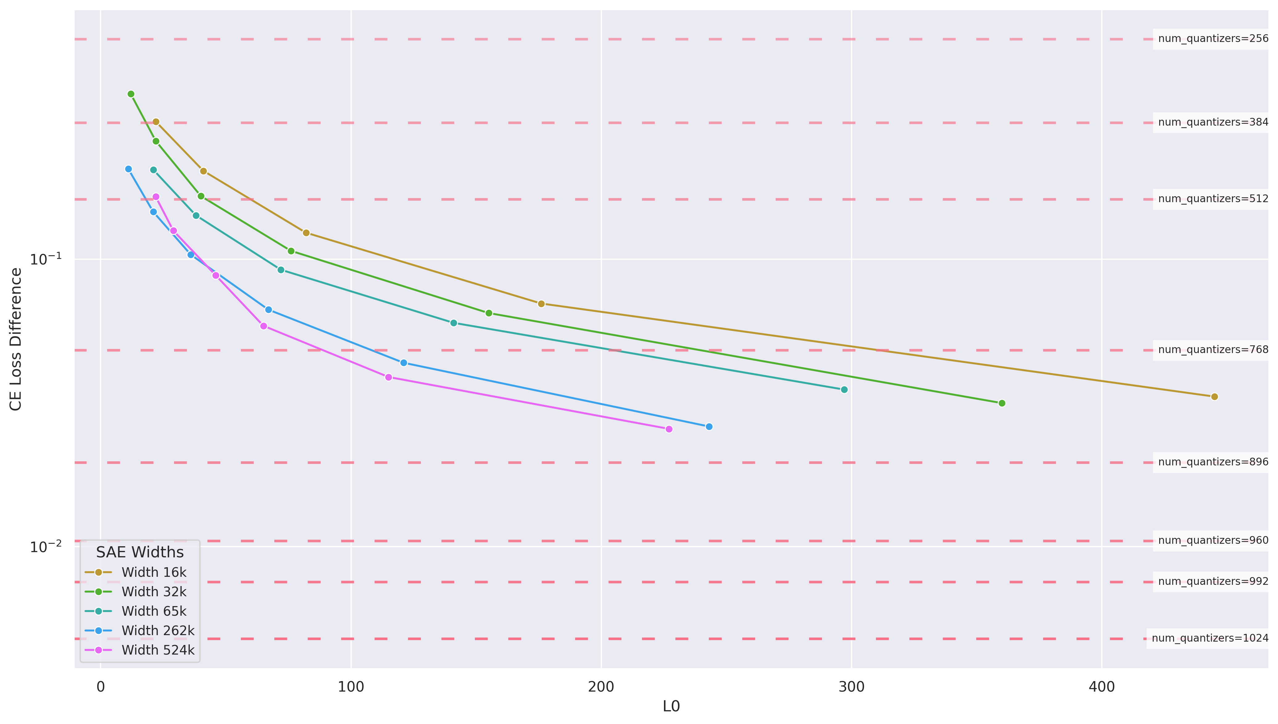
Figure 2b shows that RQAE has higher capacity (as discussed in the previous section), by reducing reconstruction loss. This is with an order of magnitude fewer parameters than an SAE (e.g. a 1M feature SAE takes up 4.6GB of space, while RQAE takes 100MB).
RQAE doesn’t have an equivalent concept of $L_0$, since all layers are used for every input. However, it still seems like an unfair comparison, since we are still using $1024$ unique vectors to reconstruct an activation with CE loss difference $< 0.01$.
The reason that we argue for this comparison is for two reasons:
- If reconstruction loss is low, then we know that we have certainly captured more of the features present in the activation (i.e. less dark matter). Higher $L_0$ may mean that the features become less interpretable in SAEs, but:
- As mentioned at the beginning of this section, the RQAE inductive bias during training does not come from sparsity. Thus, we shouldn’t expect features to be learned by sparsity, and we shouldn’t expect higher sparsity to correspond to more interpretable features.
Thus, RQAE does reduce dark matter (e.g. even a SAE with very high $L_0$ would do the same), but still learns interpretable features (as opposed to an SAE with high $L_0$). To prove the latter part of that claim, let’s first define what a feature in RQAE is.
Defining a Feature
Features in SAEs are simply defined as the columns of the decoder matrix. When a feature is present in an activation, it also has an associated intensity, measured by ($\propto$) the cosine similarity of the activation to the corresponding row in the encoder matrix. We will use this to motivate the definition of a RQAE feature. Referring back to the algorithm at the beginning of this section:
Definition 3: Let $$C_i = \{\text{codebook indices for layer }i\} = \{1,2,...\}$$ $$\mathbb{C}_i = \{\text{codebook values for layer }i\} = \{c: c \in \mathbb{R}^{codebook\_dim}\}$$ where you can index $\mathbb{C}_i$ directly with elements of $C_i$ as $\mathbb{C}_i(c)$.
Then, a RQAE feature is defined as a set of (up to) $n_{q}$ codebook indices (one per layer): $$f = [c_1, c_2, \dots, c_k]\text{ where } k <= n_{q}, c_i \in C_i$$
Definition 4: Consider a token's activation $t$, that has been quantized by RQAE (see algorithm): $$t = [t_1, t_2, t_3, \dots, t_{n_q}]\text{ where }t_i \in C_i$$ Then, the intensity of a feature $f$ in $t$ is defined as: $$C(f, t) = \frac{\sum_{i \leq k} cos\_sim(\mathbb{C}_i(t_i), \mathbb{C}_i(c_i)) \cdot L_i}{\sum L_i}$$ where $L_i$ is the average $L_2$ norm of the columns in the decoder of layer $i$ in RQAE.
Similar to SAEs, we measure cosine similarity of the activation to a set of features (only in subspaces) to measure intensity. Since we use FSQ
It’s important that RQAE uses most of the codebooks at any given layer across a large dataset. Otherwise, the model is not using different codebooks to represent different tokens, and thus measuring cosine similarity is useless. What Fig. 3a shows us is that even by layer $4$, all tokens in a reasonable large dataset can be almost completely partitioned into unique sets of codebooks.
| # Layers | 1 | 2 | 3 | 4 |
|---|---|---|---|---|
| # Used Codebooks | 544 | 234,994 | 3,279,894 | 4,383,319 |
| Average # Tokens per Codebook | 8606.1 | 19.92 | 1.43 | 1.07 |
Since RQAE is hierarchical, the number of unique sets of codebooks that RQAE learns grows exponentially with the number of layers. At first glance, this makes RQAE seem pretty useless - what’s the point of finding $544^{1024}$ new “features”?
Remember from Definition 3 that a single feature is defined by a set of codebook indices. When we choose random codebooks per layer, we get useless results, because all tokens in our evaluation dataset have nearly $0$ intensity with the feature. However, if we create a feature by choosing a token in the dataset, and creating a feature with the same codebooks as the token, that feature is highly interpretable. Having an even larger evaluation dataset would result in more unique interpretable features.
When features are defined by a set of codebooks, a natural question becomes how the feature uses each codebook. We find that more codebooks directly lead to more specific features. This makes sense given our understanding of the feature hierarchy: earlier codebooks define coarse features in the hierarchy, while later codebooks define more refined and specific features.
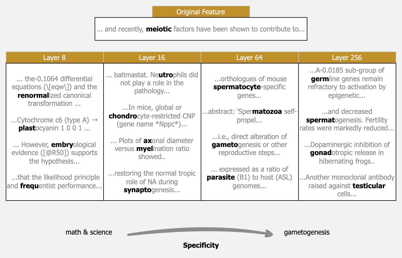
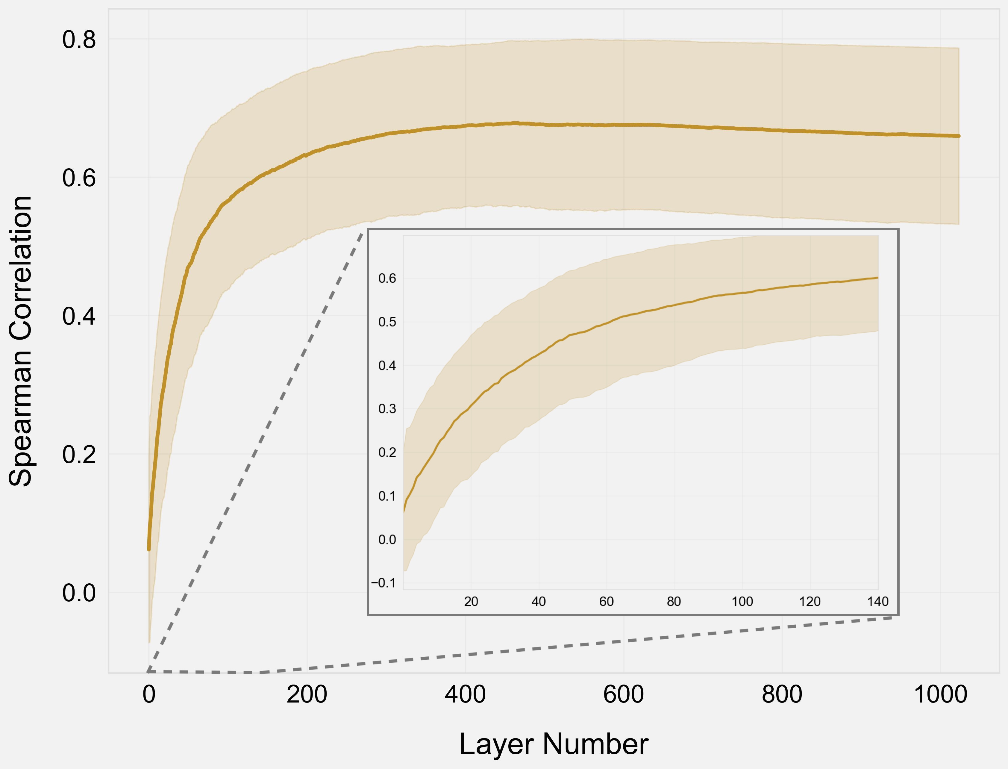
What happens when we use all $n_q$ codebooks in the model? Since RQAE has low reconstruction loss, this becomes very similar to just measuring by cosine similarity of the original activations. This means that only the dominant “feature” in the activation will be modeled, but clearly, SAEs do something similar, at least for some features. Take the Gemmascope features for any Gemmascope SAE, and a large portion (from manual checks, 30+%) of them will be single-token features (i.e. the feature only fires on a single token).
Fig. 3c shows us that earlier layers are certainly doing something different than just ranking by cosine similarity. Specifically, even up to layer $64$ we do not find the Spearman correlation to be above $0.5$, indicating a moderate-weak correlation.
Feature Splitting and Absorption
Since RQAE models the feature hierarchy, we should define how features can split and be absorbed.
Definition 3: Given a RQAE feature $f$: $$f = [c_1, c_2, \dots, c_k]$$ The ancestors of $f$ are a set of RQAE features: $$A_m(f) = \{g: g = [c_1, c_2, \dots, c_m]\}\text{ } \forall m < k$$ Two features $f_1$ and $f_2$ are considered $m$-split features if $$C(a_1, a_2) \geq \theta\text{ } \forall a_1 \in A_m(f_1), a_2 \in A_m(f_2)$$ for some threshold $\theta$.
Essentially, two features are split if some subset of their ancestors are close, but they diverge at some point. This definition does mean that features can split at one layer, and then merge later on, but we couldn’t find interesting examples of this in practice. To illustrate what this looks like, let’s look at an example:
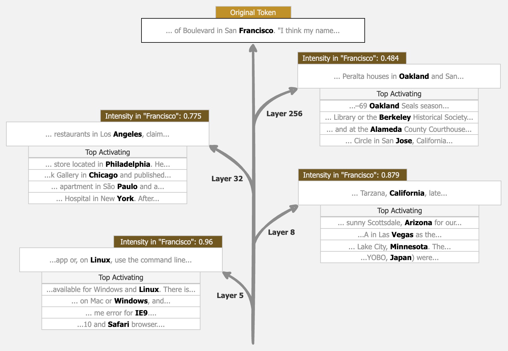
We developed heuristics for how to choose $\theta$ based on intensities on a test dataset, but we think there’s much more detail that can be added to feature splitting in RQAE - for example, learning thresholds per feature like in JumpReLUs
Comparison to Gemmascope
It’s hard to propose a new architecture, when the existing architecture already has a large body of work and empirical evidence: for example, Gemmascope
Finding Equivalent Features
SAEs are useful because they develop a dictionary of features. Although this dictionary is static after training, the small dictionary can be evaluated in depth to come to promising interpretability results.
In contrast, as mentioned above RQAE has exponentially many features - far too many to manually or even automatically interpret. Thus, it’s interesting to know if:
- The same features that an SAE finds exist in RQAE
- There is an easy way to identify those features automatically in RQAE.
To validate if a RQAE feature is “equivalent” to a SAE feature, we measure the Pearson correlation between SAE intensities and RQAE intensities on top activating, and median-activating examples of the original SAE feature. If this number is high, then the two methods generally recognize the same tokens at the same intensities, and the features are very close. This gives us a measure of determining if the same features exist in RQAE.
An easy way to identify a feature would be looking at it’s top-activating example. If, using this example, RQAE can faithfully reconstruct the feature (as defined above), then we could simply create features from every token in a dataset (which would be tractable to evaluate, e.g. the dataset we use in this work is 4M tokens), and find the most interpretable ones.
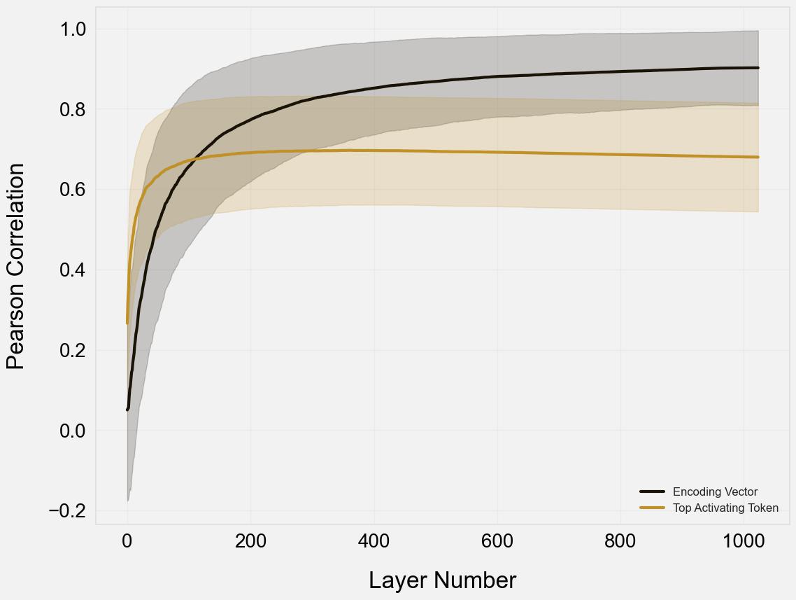
This result certainly shows that Gemmascope features exist and can be represented with RQAE, since the Pearson correlation of the encoding vector approaches $1$. This means that for every Gemmascope feature, there exists some RQAE feature which ranks tokens very similarly to it.
Using the top-activating example to create a feature, however, is a mixed result. Clearly, as expected, it underperforms using the encoding vector. However, a Pearson correlation of $0.7$ still suggests that there is a strong correlation between the two. We consider this to be good enough evidence to continue using top-activating examples to search for RQAE features, although we discuss more in the conclusion why this might need future work.
Finally, let’s qualitatively look at some examples of Gemmascope features, and how they compare to RQAE features that use their top activating example. We looked for three particularly complex features, to ensure that we don’t bias towards single-token features, which we expect RQAE to capture well already. All features were taken from the 16k SAE with $L_0=81$:
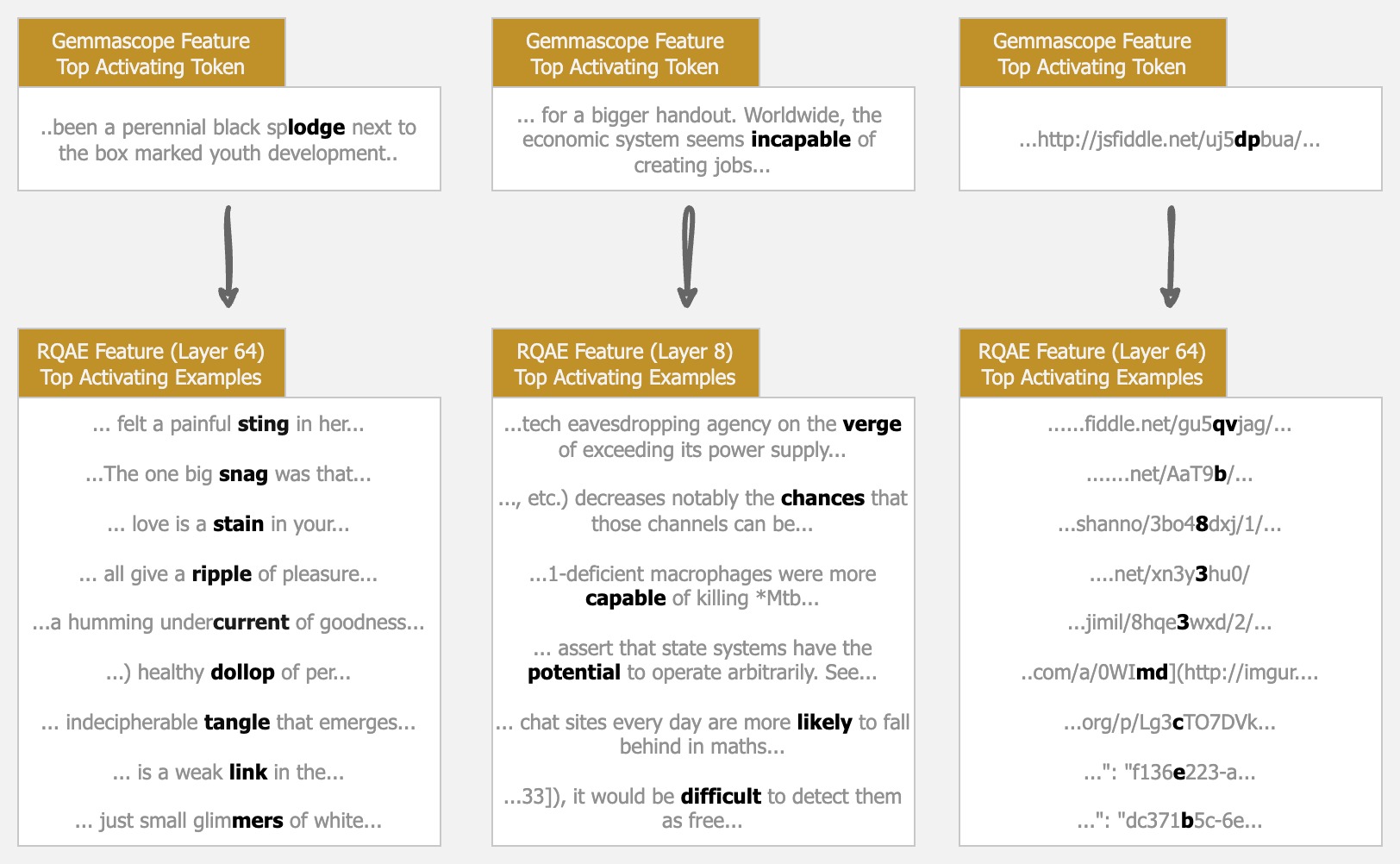
Qualitatively, even for “complex” features, it seems that RQAE does a good job of representing the feature! We talk more in the conclusion about further ideas we find interesting which stem from these results.
Evaluations
Evaluating interpretability methods is still an open problem. In this work, we will use Eleuther’s auto-interpretation suite
We perform all evaluations on the monology/pile-uncopyrighted dataset - specifically, the same subset of 36864 sequences (128 tokens each) that is also used in Neuronpedia to interpret Gemmascope SAEs. You can also see all features used, as well as the full evaluation traces, in the dashboard. As a result, you can directly compare all scores, explanations, and activating examples with Gemmascope easily.
For all evaluations, we throw out Gemmascope features without enough max-activating examples in the dataset - we do this by removing features with < bos > tokens as max-activating examples.
Creating a Dictionary of Features
To compare to SAEs, we need to actually define a single set of features. We have already motivated this method in the previous section, but to explicitly define how to make a dictionary of at least $k$ features using RQAE:
- Begin with some test dataset of tokens. We use
monology/pile-uncopyrighted. - Choose $k$ tokens with enough diversity from this dataset. We select uniformly from unique tokens.
- Create a set of $b$ RQAE features per token by using the quantized codebooks of the layer, and then choosing $b$ subsets of layers (i.e. the first 512, the first 256, the first 128, etc.)
- Optionally, filter features (we only consider layers $16$, $64$, and $256$ for evaluation).
This method is a naive approach to selecting features. However, from manual inspection it does seem to find features that are (1) unique, (2) interpretable, and (3) consistent among top-activating examples. We discuss future work for selecting features in the conclusion.
Results
There are two axes that are commonly considered to affect SAE interpretability: model width and $L_0$. We sweep across both these dimensions:
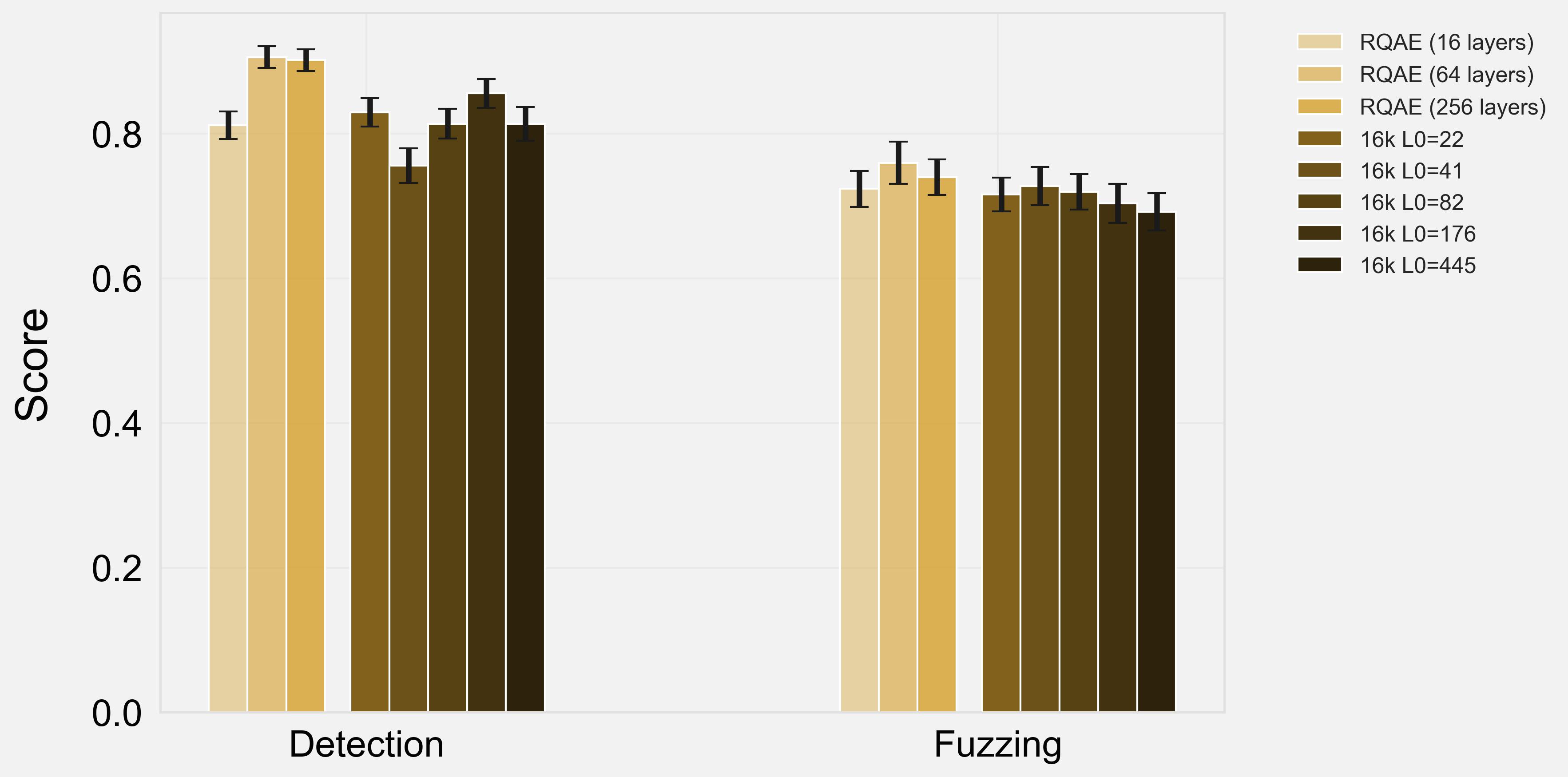
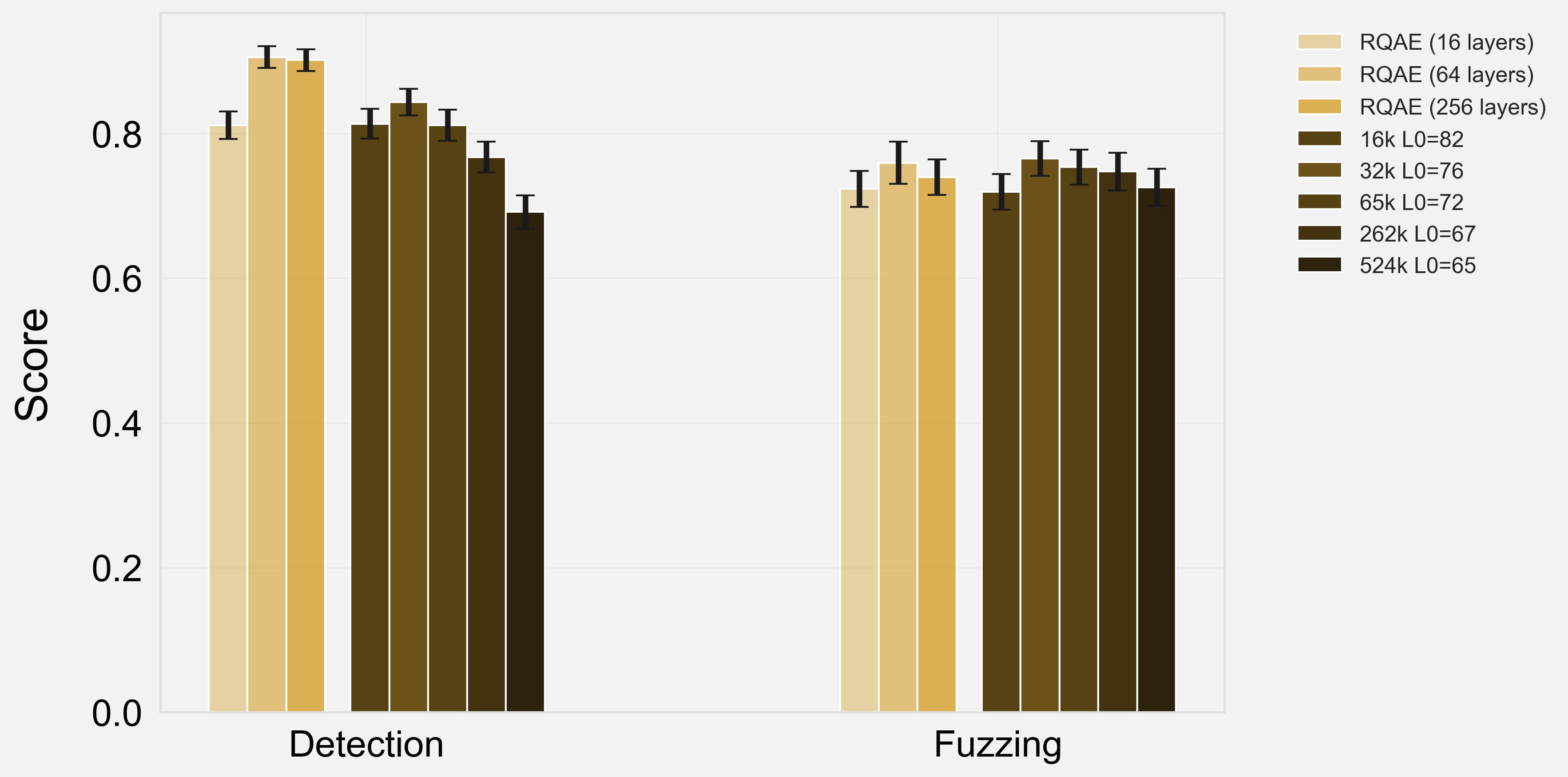
Across models and both axes, we see that RQAE generally outperforms SAEs in detection, and performs similarly in fuzzing. Generally, we see that more layers is better for RQAE, although this might saturate (e.g. $256$ layers performs the same as $64$ layers).
Using RQAE
We provide all <a href="https://www.github.com/harish-kamath/rqae">code</a> and <a href="https://huggingface.co/harish-kamath/rqae">models</a> for RQAE. We’d love to see more work being done, and this work only serves to introduce RQAE. We briefly show some interesting results using RQAE:
Feature Visualization Dashboard
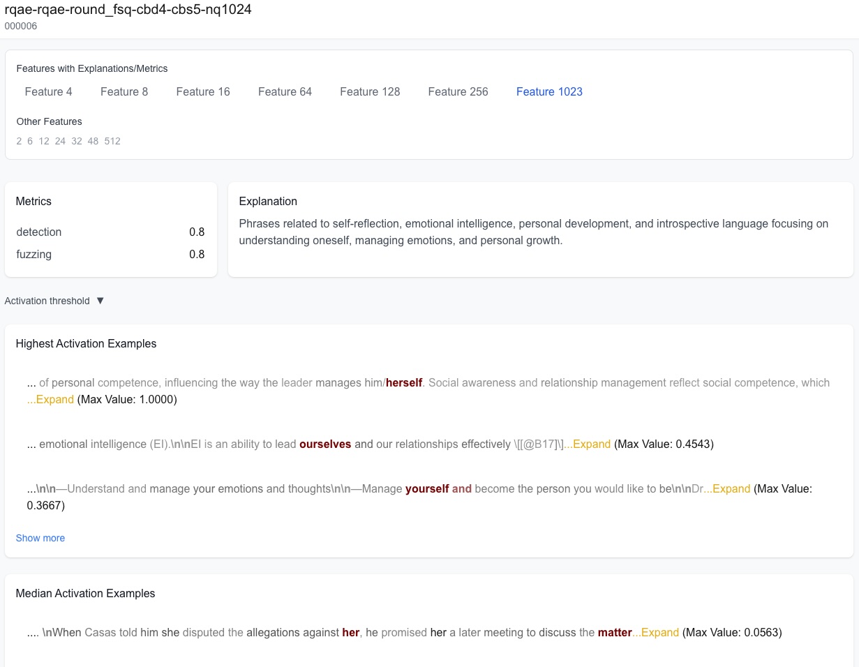
Many results in this work rely on qualitative claims by looking at specific examples of features, activations, and dataset examples. We provide a hosted visualization dashboard that contains a large number of RQAE and gemmascope features, as well as all traces from evaluations, so you can easily evaluate for yourself how well RQAE works.
Steering
We show preliminary results of steering using RQAE features. We could not find evaluations to quantitatively compare steering with SAE or activation steering - so we will leave this for future work. Steering is performed by:
- During generation, take the latest given LLM activation. Quantize it with RQAE into a set of codebooks.
- Take the codebooks of the feature you are steering with. Turn the activation codebooks towards the feature codebooks dependent on some strength $\kappa$ and the cosine similarity between the codebook and the feature’s codebook.
- Continue for all tokens during generation.
Here are some qualitative examples of steering:
Steering parameters: temperature=0.5, num_layers=5, strength=0.8, repetition_penalty=1.5
prompt="An interesting animal is the"
... know an Anglican-Catholic priest...
Steering parameters: temperature=0.5, num_layers=32, strength=0.8, repetition_penalty=1.5
prompt="An interesting thing"
... and not depressive psychosis) will...
Steering parameters: temperature=0.5, num_layers=128, repetition_penalty=1.5
prompt="Let's talk about"